FEH statistical analysis
Source:vignettes/FEH-statistical-analysis.Rmd
FEH-statistical-analysis.RmdIntroduction
This quick guide provides an overview of the core FEH functions that can be used to generate extreme flow estimates from single-site or pooling (gauged & ungauged) approaches. It is assumed that the reader has knowledge of the theory of these approaches; this guide is intended to demonstrate how to use the UKFE package rather than to explain the FEH statistical method.
The following table provides the key functions for implementing the FEH methods.
| Function | Purpose |
|---|---|
| GetCDs/CDsXML | Get catchment descriptors using the NRFA gauge reference number or import them from XML files downloaded from the FEH Web Service |
| GetAM/AMImport | Get annual maximum data from sites suitable for pooling or from AM files |
| QuickResults | Provides default pooling results (gauged, ungauged & fake ungauged), directly from catchment descriptors |
| QMED | Estimates QMED from catchment descriptors with donor options (either donor IDs or a number of donors - which are then automatically chosen based on distance) |
| DonAdj | Provides a list of donor candidates based on proximity to the study catchment |
| Pool | Creates a pooling group with the option of excluding one or more sites |
| H2 | The heterogeneity measure for pooling groups |
| DiagPlots | Provides a number of diagnostic plots to compare the sites in a pooling group |
| Zdists | The Zdist statistic to determine the distribution with the best fit to the pooling group |
| PoolEst | Flood estimates from the pooling group |
| Uncertainty | Quantifies uncertainty for gauged (enhanced single-site) and ungauged pooling groups |
| GenLog/GEV/GenPareto/Gumbel/Kappa3 | Four functions for each distribution to fit the distribution and obtain flood frequency estimates and growth factors |
| POTextract or POTt | Functions for extracting peaks over threshold data |
| AnnualStat | Extract annual statistics. The default is maximum, but any statistic can be used such as sum or mean. |
We need to load the package before we can use any of the functions:
Overview and assumptions of the FEH statistical method
This section provides a brief overview of the FEH statistical method, and its core assumptions. Examples of how to apply the method can be found later.
The FEH statistical method comes under the broader term of ‘regional frequency analysis’ and employs the “index flood” procedure for estimating peak flows at a single location on a river line. The procedure has two main steps, which are multiplied together for a final result:
Estimate the index flood (in the FEH method, the index flood is QMED - the median annual maximum flow).
Calculate the growth curve: This provides growth factors as a function of return period and is a standardised model of the AMAX distribution. In this case a growth factor is the extreme flow of interestd (such as the 100-year flow) divided by QMED.
Multiplying the index flood by the growth curve scales the standardised growth factor to produce the flow estimate for the catchment of interest. When the catchment is gauged, the index flood is estimated as the median of the observed annual maximum sample (assuming suitable data quality). When the catchment is ungauged, the index flood is estimated using a multiple regression equation, using catchment descriptors as predictors.
The growth curve is estimated by pooling gauged data from catchments which are similar to the catchment of interest. A statistical distribution is assumed. Then, weighted average parameters of the fitted distribution (L-moment ratios) from the AMAX samples in the pooling group are used to estimate the growth curve.
There are numerous choices and possible adjustments which can be made for each step. The UKFE package, in general, provides default settings with no adjustments; however, these can be changed by the user.
There are several key underlying assumptions in FEH statistical analysis. As stated in Hosking and Wallis (1997), the index-flood procedure makes the following assumptions:
Observations at any given site are identically distributed.
Observations at any given site are serially independent.
Observations at different sites are independent.
Frequency distributions at different sites are identical apart from a scale factor.
The mathematical form of the regional growth curve is correctly specified.
The first of these leads to the assumption of stationarity
(i.e. observations of past flood events are assumed to represent the
behaviour of future events). Where this is not the case, non-stationary
methods can be applied. For example, non-stationary distributions can be
fitted using other software such as the nonstat R package
(Hecht and Zitzmann, 2025).
The QMED regression equation was calibrated using an approach similar to the generalised least squares method. This allows for covariance of the model residuals (errors). Firstly, the observed QMEDs (on which it was calibrated) were logarithmically transformed. The catchment descriptors used were also transformed. With this in mind, the assumptions of the QMED equation are as follows:
The relationship between the transformed independent variables (predictors) and the logarithmically transformed dependent variable (QMED) is linear.
Observations (observed QMEDs used in calibration) are independent of each other.
Model and sampling errors are independent of each other.
Model and sampling errors are normally distributed and have a mean of zero.
Predictor variables are independent.
The cross-correlation of model errors can be described by the distance between catchment centroids, and the form of the associated correlation matrix is known for the calibration process.
Getting catchment descriptors
One of the first steps in any FEH analysis is to obtain catchment descriptors (CDs). See the ‘Data input’ article for information on functions for importing CDs.
Quick results
Once you have some catchment descriptors, you can start to use many
of the FEH based functions. The full process, covered shortly, is
encompassed in the QuickResults() function. This provides
results from a default pooling group, automatically accounts for
urbanisation, and provides a donor transfer from 8 sites by default
(this number can be adjusted). Note that if the site is gauged and in
the PeakFlowData dataframe (and the descriptors are the same) the QMED
will default to the observed QMED. The default distribution is the
generalised logistic distribution. Further details and assumptions are
provided in the function’s help file.
First, we’ll obtain some CDs for site 55002 and then apply the QuickResults function. The results from the default analysis at gauge 55002 are printed to the console. This is a list with three elements. The first is a data frame with the following columns: return period (RP), peak flow estimates (Q) and growth factor estimates (GF). The second element is the estimated L-CV and L-skew (linear coefficients of variation and skewness). The third element provides distribution parameters (location, scale, and shape) for the chosen distribution (generalised logistic by ddault).
# Get catchment descriptors for NRFA site 55002 and save to an object called CDs.55002
CDs.55002 <- GetCDs(55002)

# Obtain estimates and plots for the gauged scenario using default settings
QuickResults(CDs.55002)
#> $Results
#>      RP    Q   GF
#> 1     2  431 1.00
#> 2     5  552 1.28
#> 3    10  636 1.48
#> 4    20  725 1.68
#> 5    30  780 1.81
#> 6    50  855 1.98
#> 7    75  917 2.13
#> 8   100  965 2.24
#> 9   200 1090 2.52
#> 10  500 1270 2.95
#> 11 1000 1430 3.32
#>
#> $`Weighted Lmoment Ratios`
#>         LCV     LSKEW
#> 1 0.1792506 0.1652001
#>
#> $`Distribution Parameters`
#>        loc    scale      shape
#> 1 426.5924 79.33469 -0.1603123
Estimating QMED
There is a QMED() function which provides the ungauged
QMED (median annual maximum flow) estimate from catchment descriptors.
There is an option to adjust this using donor sites. The simplest case
is to provide catchment descriptors with no donor transfer:
# Estimate QMED from the catchment descriptors for site 55002
QMED(CDs.55002)
#> [1] 554
By default, this gives urban adjusted QMED results.
To undertake a donor transfer (with the aim of improving the
estimate), you can state how many donors you wish to apply with the
no.Donors argument (this applied the closest - by catchment centroid - n
donors). Or you can specify a vector of IDs. In which case a list of
donor site candidates is necessary. For this, there is the
DonAdj() function, which provides the closest N
gauges (default of 10) to the site (geographically by catchment
centroid) that are suitable for QMED, along with catchment
descriptors.
# Identify donor catchments based on the catchment descriptors for site 55002
DonAdj(CDs.55002)
#>          AREA ALTBAR ASPBAR ASPVAR BFIHOST19scaled BFIHOST19 BFIHOST DPLBAR
#> 55002 1894.00    297    128   0.08           0.416     0.421   0.472  95.63
#> 55007 1283.00    343    132   0.09           0.381     0.387   0.426  42.94
#> 55016  358.90    324    157   0.07           0.399     0.398   0.427  32.92
#> 55013  125.90    303    103   0.20           0.468     0.468   0.553  14.84
#> 55012  246.70    333    136   0.11           0.381     0.380   0.431  20.67
#> 56003   62.66    311    175   0.21           0.449     0.449   0.529  10.94
#> 56013   63.54    349    151   0.18           0.406     0.406   0.495  11.95
#> 55014  202.50    299    122   0.18           0.540     0.540   0.593  17.88
#> 55004   73.01    412    152   0.19           0.342     0.342   0.402  11.67
#> 55023 4016.00    227    127   0.10           0.494     0.496   0.542 130.30
#>       DPSBAR FARL2015  FARL  FPEXT    LDP PROPWET RMED.1H RMED.1D RMED.2D
#> 55002  134.4   0.9586 0.967 0.0693 157.70    0.50    10.2    42.4    56.1
#> 55007  152.4   0.9544 0.960 0.0412  84.45    0.53    10.3    44.7    60.0
#> 55016  132.2   0.9987 0.998 0.0428  62.29    0.49     9.6    36.2    48.5
#> 55013  130.1   1.0000 0.999 0.0382  28.33    0.49     9.8    37.5    48.7
#> 55012  158.6   0.9954 0.997 0.0419  39.53    0.65    10.8    50.0    66.4
#> 56003  121.0   1.0000 0.999 0.0268  21.79    0.53    10.4    43.1    56.6
#> 56013  137.9   1.0000 1.000 0.0257  23.08    0.61    10.7    45.5    59.5
#> 55014  158.5   0.9984 0.996 0.0646  31.70    0.49     9.8    36.1    47.3
#> 55004  188.7   0.9938 1.000 0.0284  23.04    0.65    11.4    52.8    70.0
#> 55023  116.1   0.9691 0.979 0.0824 244.20    0.38    10.1    38.7    50.3
#>       SAAR9120 SAAR6190 SAAR4170 SPRHOST URBEXT2015 URBEXT2000 URBEXT1990
#> 55002     1328     1230     1269   39.67     0.0049     0.0029     0.0020
#> 55007     1491     1386     1413   42.23     0.0037     0.0022     0.0010
#> 55016     1191     1066     1129   40.33     0.0059     0.0031     0.0018
#> 55013     1094      962     1086   34.31     0.0068     0.0046     0.0030
#> 55012     1722     1627     1639   42.75     0.0023     0.0020     0.0004
#> 56003     1318     1171     1257   35.20     0.0018     0.0026     0.0009
#> 56013     1476     1299     1426   38.25     0.0009     0.0003     0.0000
#> 55014     1086      977     1062   31.41     0.0060     0.0009     0.0023
#> 55004     1965     1845     1913   46.25     0.0025     0.0033     0.0009
#> 55023     1101     1010     1054   35.60     0.0110     0.0072     0.0067
#>       DrainDens  CEast CNorth    Lcv    LSkew  LKurt    L1     L2  N
#> 55002     1.196 306152 255939 0.1210  0.12100 0.0607 441.0  53.60 39
#> 55007     1.227 298496 263086 0.1840  0.21600 0.1500 574.0 106.00 84
#> 55016     1.244 309100 270212 0.0974 -0.00892 0.0581 119.0  11.50 49
#> 55013     1.116 323593 254543 0.1900  0.14000 0.1360  29.3   5.57 55
#> 55012     1.279 289404 250198 0.2090  0.12800 0.1580 200.0  41.80 55
#> 56003     1.220 302460 237118 0.2580  0.31800 0.3030  25.7   6.63 21
#> 56013     1.130 297636 238410 0.2120  0.35300 0.2960  39.8   8.46 52
#> 55014     1.169 324893 265277 0.2670  0.29600 0.1450  34.0   9.09 56
#> 55004     1.180 284963 252747 0.1590  0.25500 0.1260  61.0   9.73 45
#> 55023     1.166 326243 248368 0.1500  0.20600 0.0783 534.0  80.30 54
#>       Suitability  QMED QMEDcd Distance
#> 55002     Pooling 431.0  554.0  0.00000
#> 55007     Pooling 516.0  497.0 10.47349
#> 55016        QMED 121.0  138.0 14.57427
#> 55013     Pooling  27.9   40.9 17.49678
#> 55012        QMED 189.0  162.0 17.70465
#> 56003        QMED  23.5   31.1 19.17970
#> 56013        QMED  34.6   41.0 19.48815
#> 55014        QMED  26.7   46.9 20.93856
#> 55004     Pooling  56.5   71.6 21.42808
#> 55023        QMED 496.0  658.0 21.47017
You can apply one or multiple donors using the DonorIDs argument
within the QMED() function. Or, as noted just specify a
number of donors. The following, shows both of these. Note that the one
specifying no.Donors = 3, will default to the observed QMED because site
55002 is both the catchment of interest and the closest donor and will
have all the weighting in the adjustment. Lastly you can also output all
the detail of the donors by using the
# Estimate QMED from the catchment descriptors for site 55002 using gauges with NRFA
# IDs 55007 and 55016 as donor sites
QMED(CDs.55002, DonorIDs = c(55007, 55016, 55013))
#> [1] 510

# Use the closest three donor sites
QMED(CDs.55002, no.Donors = 3)
#> [1] 431

#Use the specified three donors and return the associated details of the adjustment
QMED(CDs.55002, DonorIDs = c(55007, 55016, 55013), ReturnDetails = TRUE)
#> $QMEDEstimate
#> [1] 510
#>
#> $DonorDetails
#>      ID     alpha ObservedQMED QMED_DeUrbanised QMEDcdRural QMEDcdUrban
#> 1 55007 0.2532231        516.0            514.0       495.0       497.0
#> 2 55016 0.1749968        121.0            120.0       137.0       138.0
#> 3 55013 0.1771742         27.9             27.6        40.4        40.8
#>   QMEDRatio Distance      UAF
#> 1     1.040    10.47 1.004590
#> 2     0.877    14.57 1.007610
#> 3     0.684    17.50 1.010217
The user should be aware of the following specifics about the UKFE implementation of QMED estimation. However, note that there is an inherent flexibility in ‘R’, so any code can be edited.
Note that the
QMEDDonEq()function can also be used, and a number of donors could be used in turn - the user would need to choose the donor weights.The
DonAdj()function only provides candidate donor sites from the NRFA “suitable for QMED and pooling” dataset. However, theQMEDDonEq()can be applied, which is entirely flexible regarding inputs.By default, the
QMED()function uses the URBEXT2015 catchment descriptor with an urban expansion (set to current year). There is an argument within the function calledUrbanExpansion, which is set toTRUE. This can be set toFALSEif required. There is also theUEF()function, which can be applied independently, and for any year.
Creating a pooling group
To create a pooling group, the Pool() function can be
used. If it is for a gauged site, the site will be automatically
included in the group, unless it is has an URBEXt2015 above UrbMax
(default 0.03). If you wish to include the urban site, the
include argument can be set be used (just put in the gauge
ID). Alternatively UrbMax can be increased (note that this will allow
other ubran sites into the group). There is a DeUrb
argument which is TRUE by default. It de-urbanises the LCVs
of site in the pooling group. To create and view the pooling group:
# Create a pooling group based on the catchment descriptors for site 55002 and
# save to an object called Pool.55002
Pool.55002 <- Pool(CDs = CDs.55002)

# View the pooling group
Pool.55002
#>         AREA SAAR9120 FARL2015  FPEXT BFIHOST19scaled URBEXT2015       Lcv
#> 55002 1894.0     1328   0.9586 0.0693           0.416     0.0049 0.1213805
#> 8010  1746.0     1342   0.9377 0.0612           0.415     0.0019 0.1752132
#> 54005 2027.0     1250   0.9788 0.0919           0.439     0.0090 0.1387981
#> 21006 1506.0     1337   0.9629 0.0443           0.438     0.0043 0.1875159
#> 76007 2276.0     1316   0.9705 0.0741           0.486     0.0145 0.1998481
#> 12002 1833.0     1230   0.9804 0.0483           0.452     0.0024 0.1552385
#> 8006  2852.0     1249   0.9593 0.0525           0.433     0.0023 0.1762596
#> 84003 1093.0     1364   0.9597 0.0645           0.405     0.0067 0.1546625
#> 12001 1380.0     1270   0.9752 0.0468           0.451     0.0015 0.2232144
#> 76017 1372.0     1430   0.9536 0.0615           0.488     0.0090 0.2856425
#> 8005  1261.0     1439   0.9161 0.0589           0.402     0.0018 0.2292643
#> 84018  938.4     1402   0.9544 0.0616           0.400     0.0049 0.1755503
#> 55007 1283.0     1491   0.9544 0.0412           0.381     0.0037 0.1844367
#>        LSkew  LKurt QMED  N    SDM Discordancy Discordant
#> 55002 0.1210 0.0607  431 39 0.0000      1.4600      FALSE
#> 8010  0.0981 0.0908  241 72 0.2628      0.5300      FALSE
#> 54005 0.0385 0.1280  304 72 0.5002      0.9540      FALSE
#> 21006 0.2030 0.1600  397 63 0.5102      0.0484      FALSE
#> 76007 0.2250 0.2210  646 57 0.5294      0.5100      FALSE
#> 12002 0.0323 0.1210  556 33 0.5391      1.1400      FALSE
#> 8006  0.1580 0.1170  504 72 0.5418      0.0986      FALSE
#> 84003 0.2450 0.1970  283 69 0.5668      1.5500      FALSE
#> 12001 0.1670 0.2360  446 95 0.5942      1.6900      FALSE
#> 76017 0.3720 0.2270  494 22 0.6298      2.1200      FALSE
#> 8005  0.2070 0.0473  172 73 0.6524      2.4100      FALSE
#> 84018 0.2150 0.1790  248 56 0.7404      0.3290      FALSE
#> 55007 0.2160 0.1500  516 84 0.7462      0.1640      FALSE
You may now wish to assess the group for heterogeneity and see which
distribution fits best. The H2() function can be used to
check for heterogeneity.
# Check for heterogeneity
H2(Pool.55002)
#> [1] "1.41"                "Group is homogenous"
This group appears to be homogeneous, but if a group is
heterogeneous, you may wish to use the DiagPlots() function
to check for any outliers etc. You can also look at the discordancy
measures, which can be found in the last two columns of the pooling
group created.
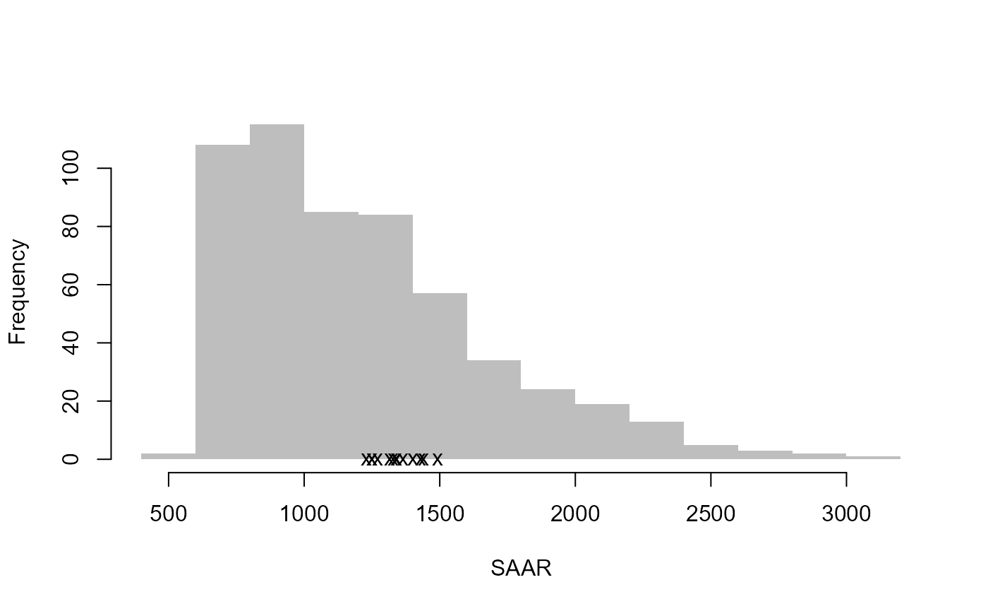
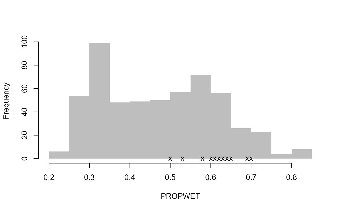
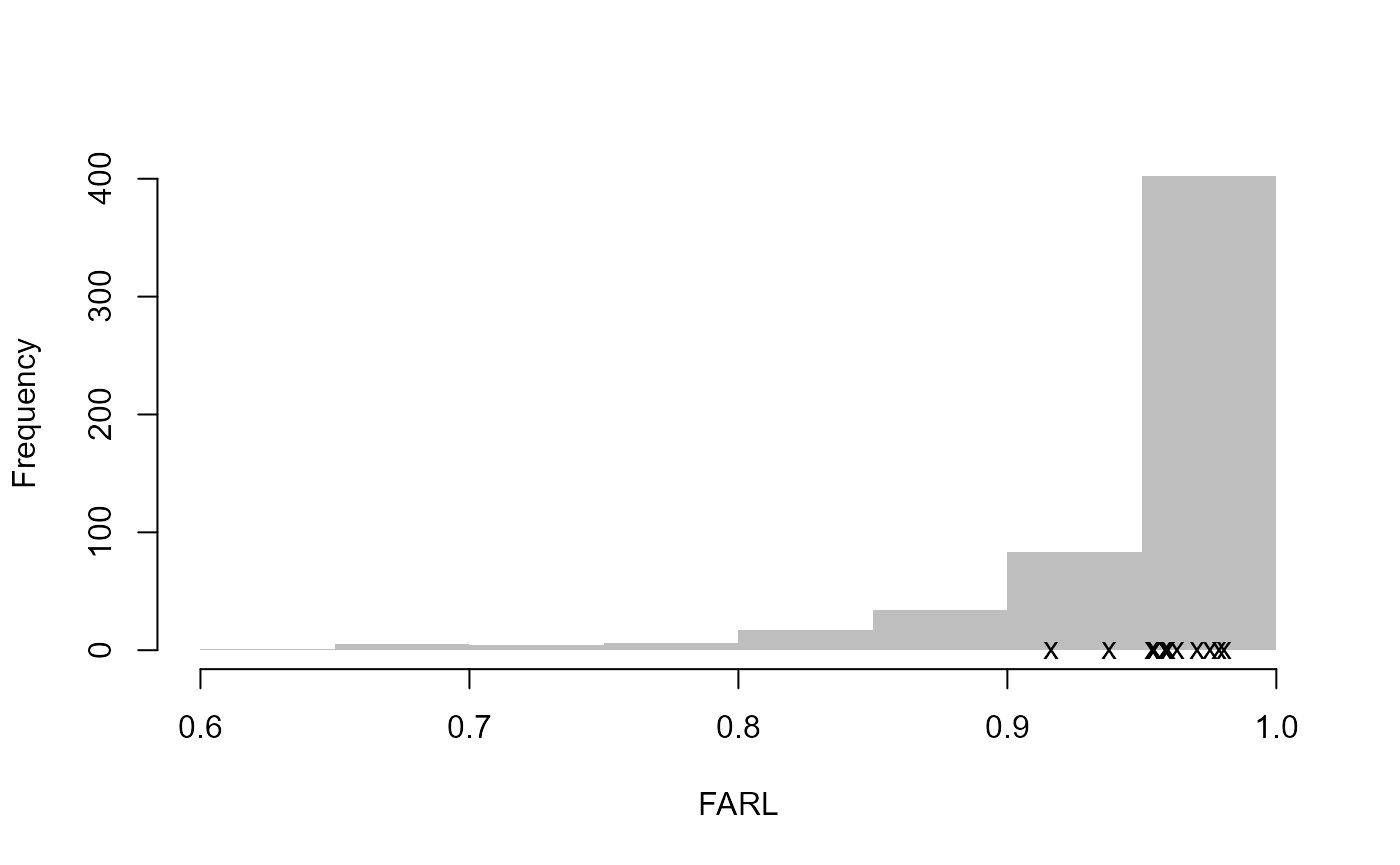
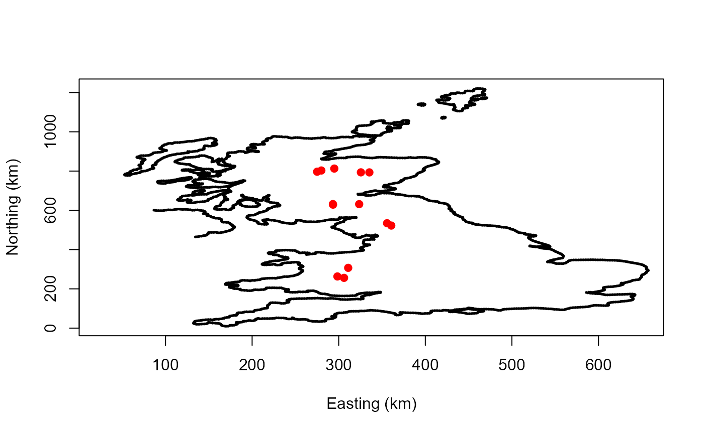
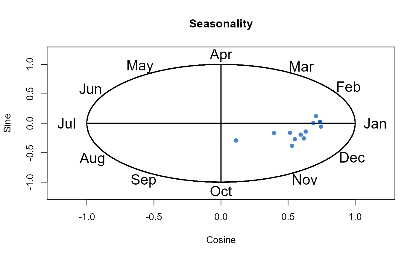
# Create diagnostic plots to aid review of the pooling group
DiagPlots(Pool.55002)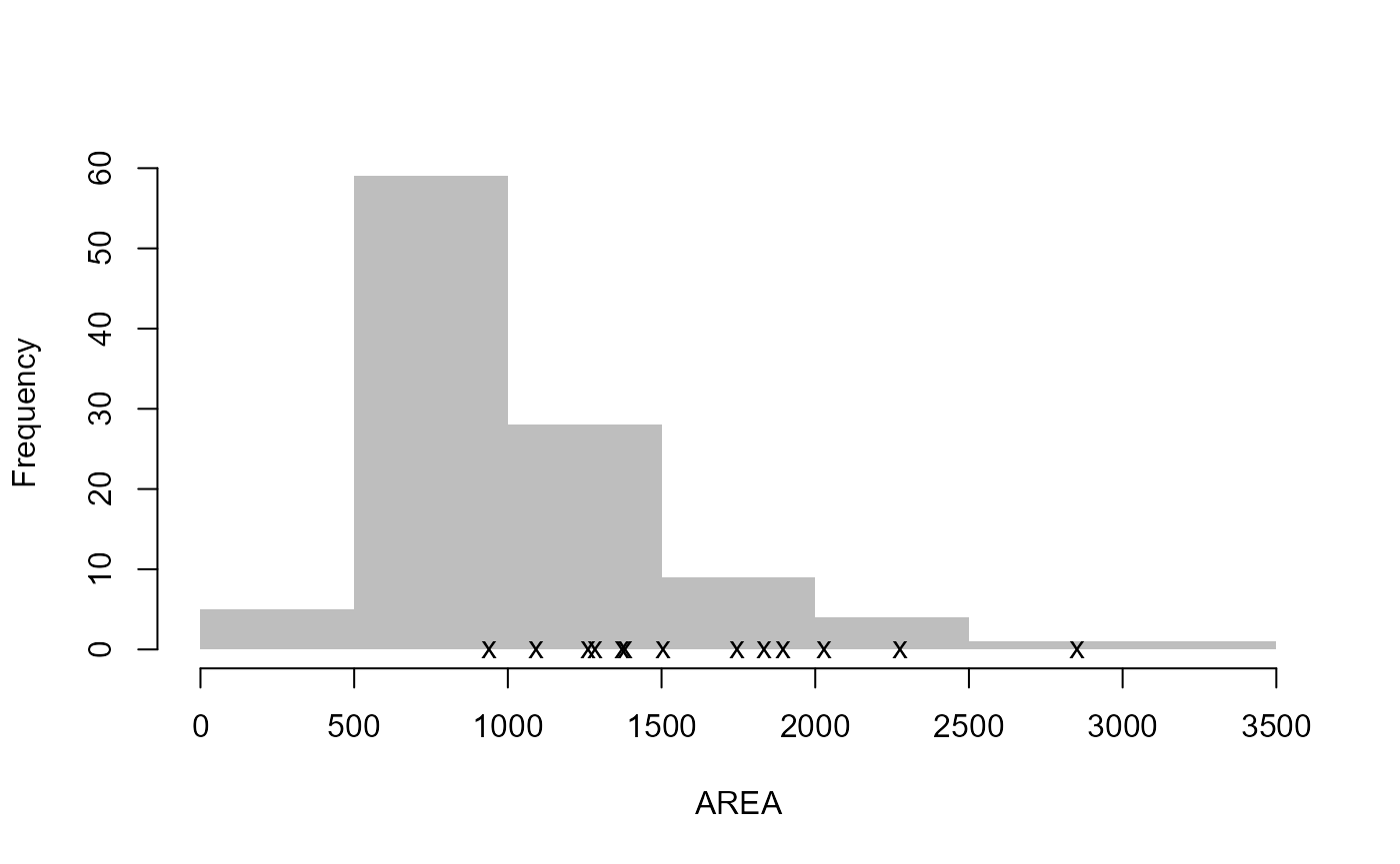
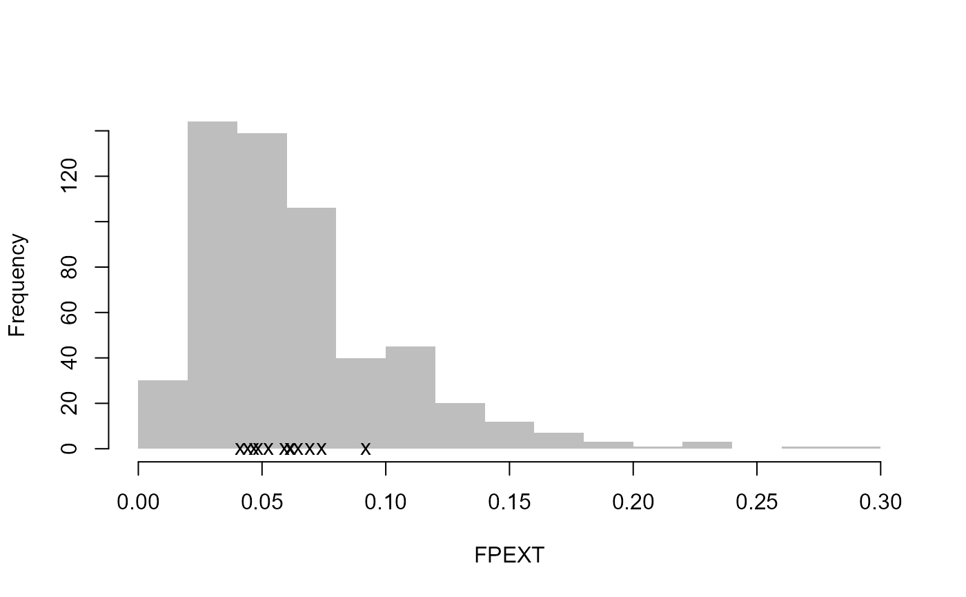
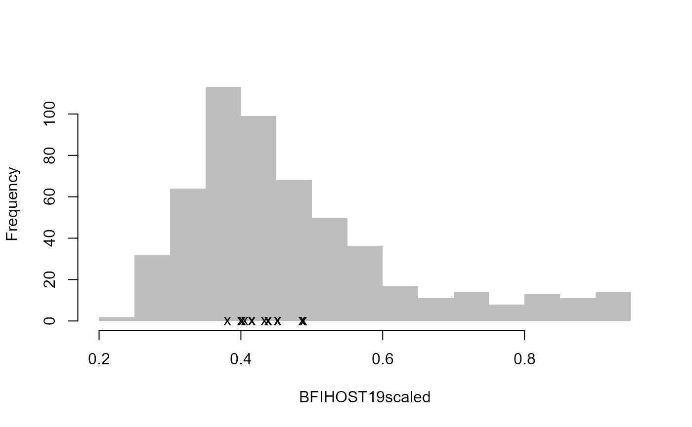
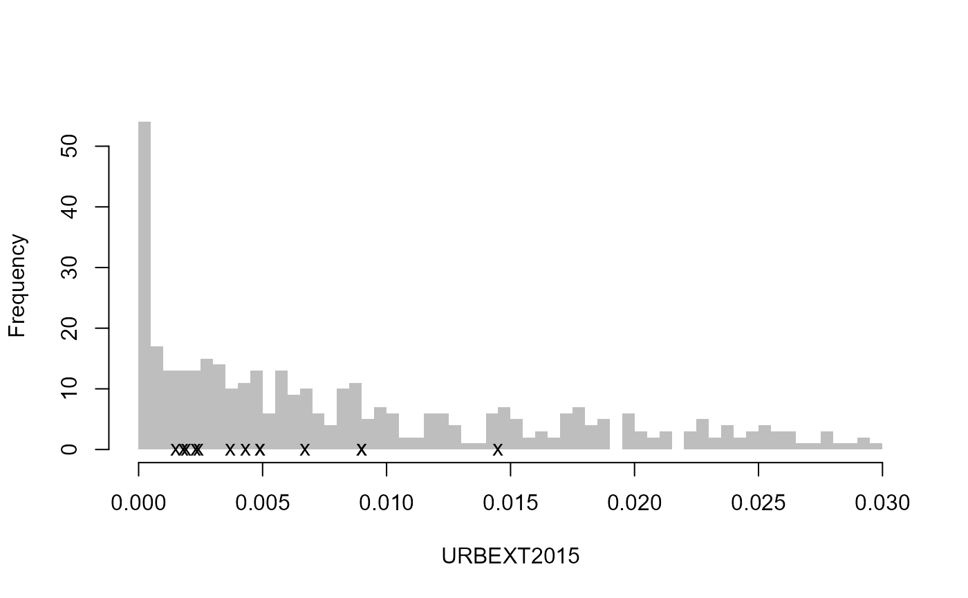
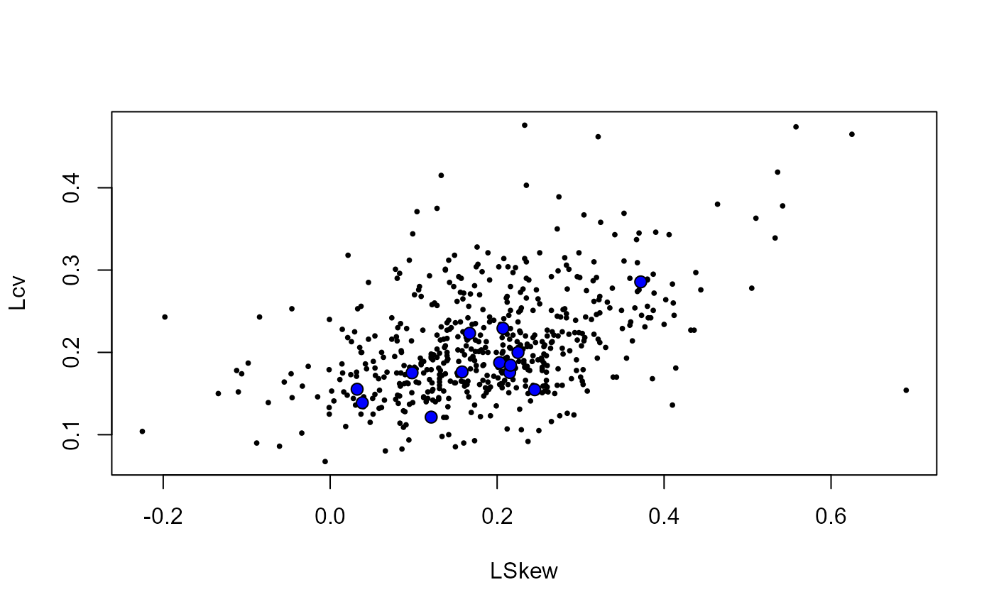
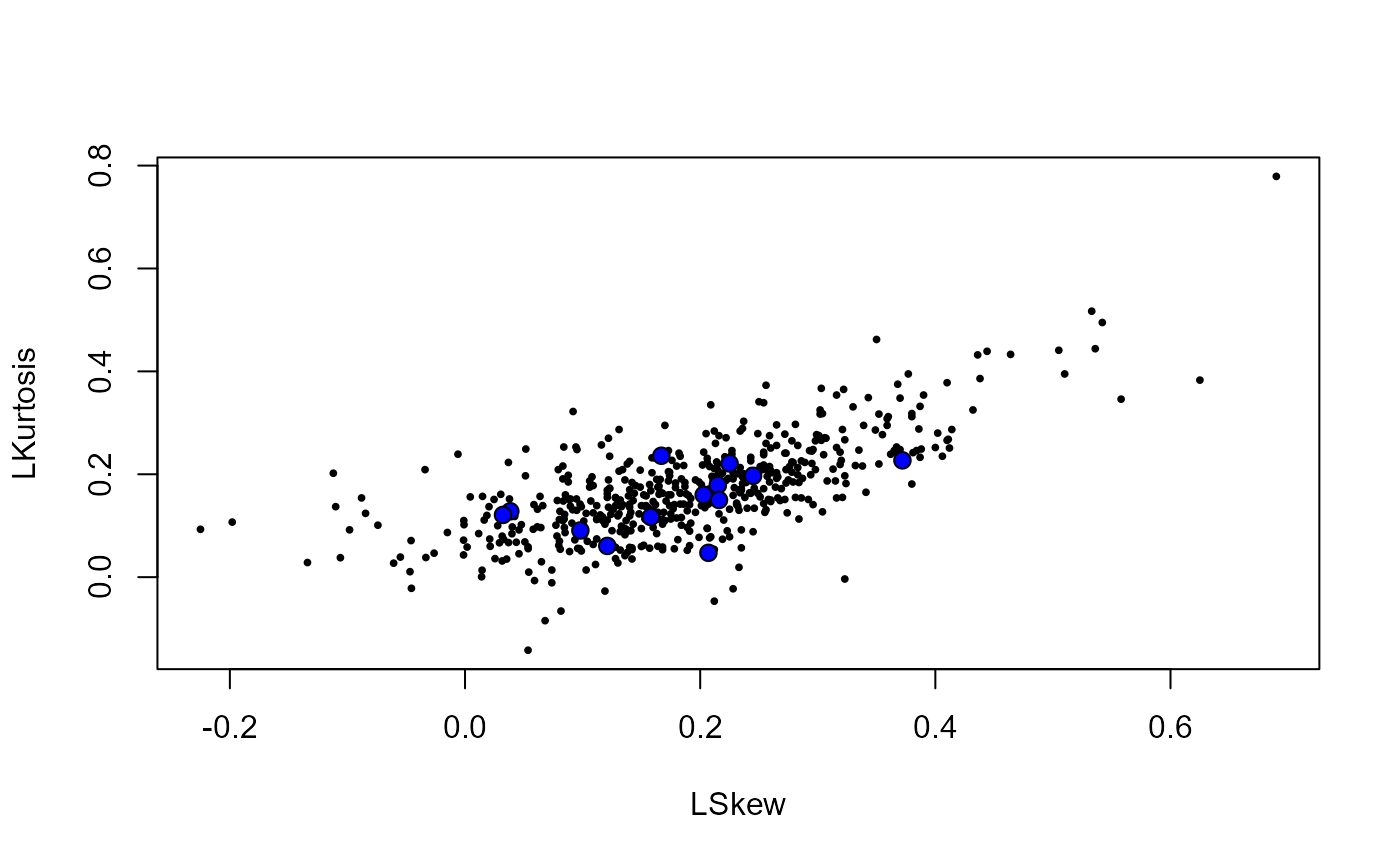
Let’s pretend that site 8010 and site 76017 are to be removed
(because they have the highest discordancy - in reality, a more thorough
analysis would be undertaken). To remove the sites, we recreate the
pooling group and use the exclude option. The function
automatically adds the next site(s) with the lowest similarity distance
measure if the total number of years of AMAX in the group has dropped
below 500 (or whatever we set as the N argument in the
Pool() function, which has a default of 800).
# Recreate the pooling group, excluding NRFA sites 8010 and 76017
Pool.55002 <- Pool(CDs = CDs.55002, exclude = c(8010, 76017))

# View the new pooling group
Pool.55002
#>         AREA SAAR9120 FARL2015  FPEXT BFIHOST19scaled URBEXT2015       Lcv
#> 55002 1894.0     1328   0.9586 0.0693           0.416     0.0049 0.1213805
#> 54005 2027.0     1250   0.9788 0.0919           0.439     0.0090 0.1387981
#> 21006 1506.0     1337   0.9629 0.0443           0.438     0.0043 0.1875159
#> 76007 2276.0     1316   0.9705 0.0741           0.486     0.0145 0.1998481
#> 12002 1833.0     1230   0.9804 0.0483           0.452     0.0024 0.1552385
#> 8006  2852.0     1249   0.9593 0.0525           0.433     0.0023 0.1762596
#> 84003 1093.0     1364   0.9597 0.0645           0.405     0.0067 0.1546625
#> 12001 1380.0     1270   0.9752 0.0468           0.451     0.0015 0.2232144
#> 8005  1261.0     1439   0.9161 0.0589           0.402     0.0018 0.2292643
#> 84018  938.4     1402   0.9544 0.0616           0.400     0.0049 0.1755503
#> 55007 1283.0     1491   0.9544 0.0412           0.381     0.0037 0.1844367
#> 27007  912.6     1223   0.9732 0.0674           0.391     0.0088 0.2041479
#> 21021 3346.0     1169   0.9746 0.0460           0.437     0.0063 0.1646634
#>        LSkew  LKurt QMED  N    SDM Discordancy Discordant
#> 55002 0.1210 0.0607  431 39 0.0000       1.750      FALSE
#> 54005 0.0385 0.1280  304 72 0.5002       1.340      FALSE
#> 21006 0.2030 0.1600  397 63 0.5102       0.123      FALSE
#> 76007 0.2250 0.2210  646 57 0.5294       0.767      FALSE
#> 12002 0.0323 0.1210  556 33 0.5391       1.450      FALSE
#> 8006  0.1580 0.1170  504 72 0.5418       0.061      FALSE
#> 84003 0.2450 0.1970  283 69 0.5668       1.570      FALSE
#> 12001 0.1670 0.2360  446 95 0.5942       2.060      FALSE
#> 8005  0.2070 0.0473  172 73 0.6524       2.290      FALSE
#> 84018 0.2150 0.1790  248 56 0.7404       0.375      FALSE
#> 55007 0.2160 0.1500  516 84 0.7462       0.229      FALSE
#> 27007 0.1810 0.0729  278 54 0.8078       0.869      FALSE
#> 21021 0.1310 0.1440  766 55 0.8146       0.120      FALSE

# Check for heterogeneity
H2(Pool.55002)
#> [1] "0.626"               "Group is homogenous"
Choosing a distribution.
Once you are happy with the pooling group, you can check for the best
distribution. The Zdists() function can be used to do this.
This compares the Generalised Extreme Value (GEV), Generalised logistic
(GenLog), Gumbel, and Kappa3 distributions. The method behind it is
outlined in Hosking and Wallis (1997). Note that it is not the same as
the method detailed in Science Report SC050050 (Kjeldsen et
al., 2008). The difference is described in the function’s help file
and is necessary to encompass the two-parameter Gumbel distribution.
# Calculate goodness-of-fit measure
Zdists(Pool.55002)
#> [[1]]
#>      GEV GenLog Gumbel Kappa3
#> 1 -0.216  -2.55 -0.213  -1.64
#>
#> [[2]]
#> [1] "Gumbel has the best fit"
The output is a list, where the first element contains the Z-scores for each distribution, and the second element states which distribution has the best fit.
The L-CV and L-skew for each site are provided in the pooling group
and are derived from the AMAX data. If the user has further information,
for example, an extra year of data to provide a new annual maximum, the
L-CV and L-skew can be calculated using the Lcv() &
LSkew() functions. The user’s data can be pasted in or read
into the ‘R’ environment. Data can be read in using a function such as
read.csv(), or a column of data can be pasted in from Excel
by running the following code and then pressing “Ctrl+V” in the console
(assuming you have already copied the required data):
MyData <- scan()This creates a numeric vector called MyData that
contains your flow data. The Lcv() &
LSkew() functions take a numeric vector of flows as their
only input, so you can then use Lcv(MyData) and
LSkew(MyData) to derive the L-moment ratios.
The relevant results can be updated in the pooling group by applying
the LRatioChange() function. For example, if you wanted a
new pooling group with updated L-moment ratios for site 55002, the
following code could be used:
# Update the pooling group to use user-supplied L-CV and L-skew values for site 55002
UpdatedPool <- LRatioChange(Pool.55002, SiteID = 55002, lcv = 0.187, lskew = 0.164)

# View the updated pooling group
UpdatedPool
#>         AREA SAAR9120 FARL2015  FPEXT BFIHOST19scaled URBEXT2015       Lcv
#> 55002 1894.0     1328   0.9586 0.0693           0.416     0.0049 0.1870000
#> 54005 2027.0     1250   0.9788 0.0919           0.439     0.0090 0.1387981
#> 21006 1506.0     1337   0.9629 0.0443           0.438     0.0043 0.1875159
#> 76007 2276.0     1316   0.9705 0.0741           0.486     0.0145 0.1998481
#> 12002 1833.0     1230   0.9804 0.0483           0.452     0.0024 0.1552385
#> 8006  2852.0     1249   0.9593 0.0525           0.433     0.0023 0.1762596
#> 84003 1093.0     1364   0.9597 0.0645           0.405     0.0067 0.1546625
#> 12001 1380.0     1270   0.9752 0.0468           0.451     0.0015 0.2232144
#> 8005  1261.0     1439   0.9161 0.0589           0.402     0.0018 0.2292643
#> 84018  938.4     1402   0.9544 0.0616           0.400     0.0049 0.1755503
#> 55007 1283.0     1491   0.9544 0.0412           0.381     0.0037 0.1844367
#> 27007  912.6     1223   0.9732 0.0674           0.391     0.0088 0.2041479
#> 21021 3346.0     1169   0.9746 0.0460           0.437     0.0063 0.1646634
#>        LSkew  LKurt QMED  N    SDM Discordancy Discordant
#> 55002 0.1640 0.0607  431 39 0.0000       1.750      FALSE
#> 54005 0.0385 0.1280  304 72 0.5002       1.340      FALSE
#> 21006 0.2030 0.1600  397 63 0.5102       0.123      FALSE
#> 76007 0.2250 0.2210  646 57 0.5294       0.767      FALSE
#> 12002 0.0323 0.1210  556 33 0.5391       1.450      FALSE
#> 8006  0.1580 0.1170  504 72 0.5418       0.061      FALSE
#> 84003 0.2450 0.1970  283 69 0.5668       1.570      FALSE
#> 12001 0.1670 0.2360  446 95 0.5942       2.060      FALSE
#> 8005  0.2070 0.0473  172 73 0.6524       2.290      FALSE
#> 84018 0.2150 0.1790  248 56 0.7404       0.375      FALSE
#> 55007 0.2160 0.1500  516 84 0.7462       0.229      FALSE
#> 27007 0.1810 0.0729  278 54 0.8078       0.869      FALSE
#> 21021 0.1310 0.1440  766 55 0.8146       0.120      FALSE
Final estimates (the growth curve and results)
To derive the final estimates, the PoolEst() function
can be applied to the pooling group. It is necessary to provide an input
for the QMED argument. Therefore, we will first obtain a
QMED estimate (in this case, we will use the data available from the
NRFA). To estimate QMED, we can either use the GetAM()
function and assess the data manually, or we can get it more directly
from the PeakFlowData data frame embedded within the
package (these are calculated as the median of the AMAX data (rejected
years excluded) from the NRFA Peak Flow Dataset). The following code
provides the latter.
# Extract QMED from the QMEDdata data frame within the UKFE package
GetQMED(55002)
#> [1] 431
We can use functions within functions so we can include the above in
PoolEst() (two things to note; we need to include the CDs
and the Gauged = TRUE argument only impacts the uncertainty
calculation):
# Derive the growth curve and final flow estimates based on the pooling group and QMED
PoolEst(Pool.55002, CDs = CDs.55002, QMED = GetQMED(55002), Gauged = TRUE)
#> $Results
#>      RP    Q   GF    FSE
#> 1     2  431 1.00 1.0623
#> 2     5  549 1.27 1.0627
#> 3    10  632 1.47 1.0641
#> 4    20  718 1.67 1.0666
#> 5    30  772 1.79 1.0687
#> 6    50  844 1.96 1.0721
#> 7    75  905 2.10 1.0753
#> 8   100  950 2.20 1.0779
#> 9   200 1070 2.48 1.0852
#> 10  500 1250 2.89 1.0970
#> 11 1000 1400 3.24 1.1073
#>
#> $`Weighted Lmoment Ratios`
#>         LCV    LSKEW
#> 1 0.1760846 0.161419
#>
#> $`Distribution Parameters`
#>        loc    scale      shape
#> 1 430.6703 76.19951 -0.1622549
The results are printed to the console. This is a list with three elements. The first is a data frame with the following columns: return period (RP), peak flow estimates (Q), growth factor estimates (GF), and factorial standard error. The latter is calculating by bootstrapping the pooling group and sampling from the QMED uncertainty. The second element is the estimated pooled L-CV and L-skew (linear coefficients of variation and skewness). The third element provide parameters (location, scale, and, shape) for the chosen distribution.
The user should be aware of the following specifics about how UKFE employs the pooled method:
The default QMED FSE is set to 1.5. This value represents the factorial standard error associated with the combined model and sampling uncertainty of the QMED model. You can update QMED FSE with the fseQMED argument. Generally it should be lower if donor catchments are applied or if the QMED is estimated from a gauged sample.
The default distribution applied is the generalised logistic distribution.
The final FSE comprises the FSE associated with QMED estimation and growth curve estimation. The FSE associated with the growth curve quantifies sampling error (aleatoric uncertainty) only. The FSE associated with QMED includes model uncertainty. In general, the uncertainty associated with the modelling process or the hydrometric data collection is not included in the FSE. Many choices are made during the process, and deriving a range of results from a range of justifiable choices is a way to quantify some of the epistemic uncertainty.
By default, urban adjustment is applied. The user can change this with the
UrbAdjargument, by setting it toFALSE.
The EVPool() function can be used to plot a growth
curve.
# Plot the growth curve
EVPool(Pool.55002, gauged = TRUE)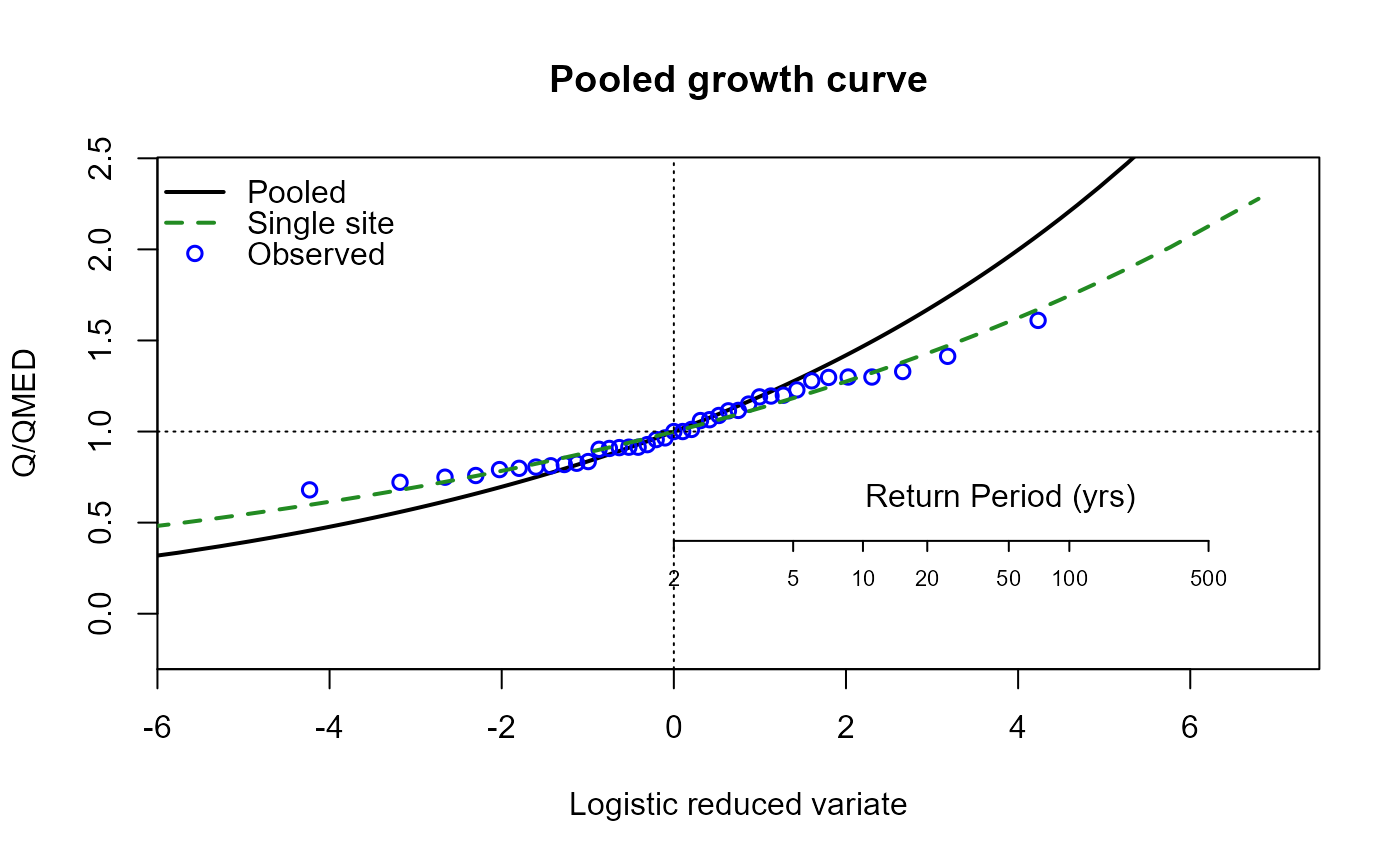
For the ungauged catchment, the same process can be followed. First, we’ll exclude the site from our pooling group. We will assume we went through a rigorous pooling group analysis and concluded all was well:
# Recreate the pooling group, excluding NRFA gauge 55002 to make it an ungauged analysis
PoolUG.55002 <- Pool(CDs.55002, exclude = 55002)

# View the new pooling group
PoolUG.55002
#>         AREA SAAR9120 FARL2015  FPEXT BFIHOST19scaled URBEXT2015       Lcv
#> 8010  1746.0     1342   0.9377 0.0612           0.415     0.0019 0.1752132
#> 54005 2027.0     1250   0.9788 0.0919           0.439     0.0090 0.1387981
#> 21006 1506.0     1337   0.9629 0.0443           0.438     0.0043 0.1875159
#> 76007 2276.0     1316   0.9705 0.0741           0.486     0.0145 0.1998481
#> 12002 1833.0     1230   0.9804 0.0483           0.452     0.0024 0.1552385
#> 8006  2852.0     1249   0.9593 0.0525           0.433     0.0023 0.1762596
#> 84003 1093.0     1364   0.9597 0.0645           0.405     0.0067 0.1546625
#> 12001 1380.0     1270   0.9752 0.0468           0.451     0.0015 0.2232144
#> 76017 1372.0     1430   0.9536 0.0615           0.488     0.0090 0.2856425
#> 8005  1261.0     1439   0.9161 0.0589           0.402     0.0018 0.2292643
#> 84018  938.4     1402   0.9544 0.0616           0.400     0.0049 0.1755503
#> 55007 1283.0     1491   0.9544 0.0412           0.381     0.0037 0.1844367
#> 27007  912.6     1223   0.9732 0.0674           0.391     0.0088 0.2041479
#>        LSkew  LKurt QMED  N    SDM Discordancy Discordant
#> 8010  0.0981 0.0908  241 72 0.2628       0.474      FALSE
#> 54005 0.0385 0.1280  304 72 0.5002       1.020      FALSE
#> 21006 0.2030 0.1600  397 63 0.5102       0.080      FALSE
#> 76007 0.2250 0.2210  646 57 0.5294       0.505      FALSE
#> 12002 0.0323 0.1210  556 33 0.5391       1.130      FALSE
#> 8006  0.1580 0.1170  504 72 0.5418       0.156      FALSE
#> 84003 0.2450 0.1970  283 69 0.5668       1.880      FALSE
#> 12001 0.1670 0.2360  446 95 0.5942       2.120      FALSE
#> 76017 0.3720 0.2270  494 22 0.6298       2.330      FALSE
#> 8005  0.2070 0.0473  172 73 0.6524       1.850      FALSE
#> 84018 0.2150 0.1790  248 56 0.7404       0.427      FALSE
#> 55007 0.2160 0.1500  516 84 0.7462       0.255      FALSE
#> 27007 0.1810 0.0729  278 54 0.8078       0.776      FALSE

# Estimate QMED from the catchment descriptors with two donors (note that the QMED
# value needs to be extracted using `$QMEDs.adj` as there are three elements to the
# output when two donors are used and the PoolEst function expects just the QMED value)
CDsQmed.55002 <- QMED(CDs.55002, DonorIDs = c(55007, 55016))

# Use the pooling group and the ungauged QMED estimate to provide the pooled estimates
Results55002 <- PoolEst(PoolUG.55002, QMED = CDsQmed.55002, CDs = CDs.55002)

# Print the results
Results55002
#> $Results
#>      RP    Q   GF    FSE
#> 1     2  544 1.00 1.5000
#> 2     5  704 1.29 1.5043
#> 3    10  817 1.50 1.5146
#> 4    20  937 1.72 1.5309
#> 5    30 1010 1.86 1.5436
#> 6    50 1110 2.05 1.5632
#> 7    75 1200 2.20 1.5818
#> 8   100 1260 2.32 1.5967
#> 9   200 1430 2.63 1.6384
#> 10  500 1690 3.10 1.7069
#> 11 1000 1910 3.51 1.7689
#>
#> $`Weighted Lmoment Ratios`
#>         LCV     LSKEW
#> 1 0.1870044 0.1743021
#>
#> $`Distribution Parameters`
#>        loc    scale      shape
#> 1 538.5441 103.6098 -0.1715526

# Plot a growth curve for the pooling group
EVPool(PoolUG.55002)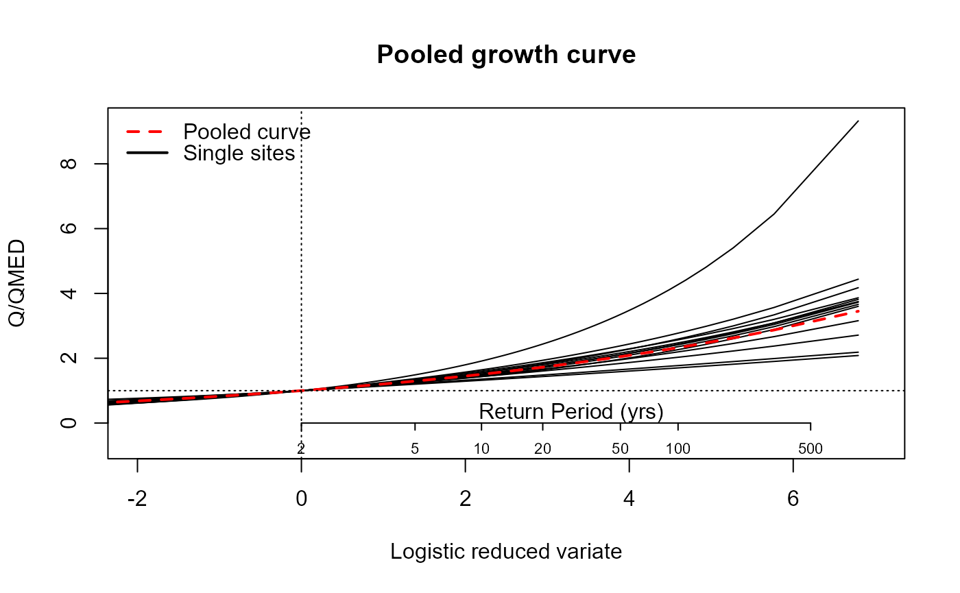
The same results are provided as for the gauged case.
Single site analysis
The quickest way to get results for a single sample are the
GEV(), GenLog(), Kappa3(),
Gumbel() and GenPareto() functions. For
example, the following code can be used to obtain a 75-year return
period estimate for an AMAX sample called MyAMAX using the
generalised logistic distribution:
GenLogAM(MyAMAX, RP = 75)An annual maximum series can be obtained for sites suitable for
pooling and QMED using the GetAM(). The
AMImport() or GetDataNRFA functions can also be used (see
the ‘Data input’ article). We will retrieve and plot the AMAX for our
site 55002:
# Extract the AMAX data for NRFA site 55002
AM.55002 <- GetAM(55002)

# View the head of the AMAX series
head(AM.55002)
#>         Date Flow    id
#> 1 1985-12-22  400 55002
#> 2 1986-11-20  457 55002
#> 3 1988-01-03  393 55002
#> 4 1989-03-24  360 55002
#> 5 1990-02-08  481 55002
#> 6 1991-01-10  412 55002

# Plot the AMAX data
AMplot(AM.55002)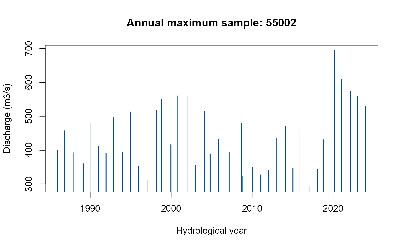
The AMplot() function returns a bar plot of the AMAX
series.
There are four functions for each of the GEV, GenLog, Gumbel, Kappa3,
and GenPareto distributions. In the function names below,
XXX should be replaced by the distribution prefix
(GEV, GenLog, Gumbel,
Kapp3, or GenPareto). For the Generalised
Pareto distribution, the first function is named
GenParetoPOT() instead of GenParetoAM().
XXXAM()- estimates return levels or return periods directly from an AMAX (or POT for GenPareto) series.XXXEst()- estimates return levels or return periods from user-supplied parameters.XXXGF()- provides the growth factor as a function of L-CV, L-skew, and RP (the Gumbel version only requires the L-CV and RP).XXXPars- estimates distribution parameters from an AMAX or POT series (using L-moments, or MLE in some cases).
We can look at the fit of the distributions using the
ERPlot() or EVPlot() functions. By default,
ERPlot() compares the percentage difference between
simulated results with the observed for each rank of the data. Another
option (see the ERType argument) compares the simulated
flows for each rank of the sample with the observed flows of the same
rank. For both plots, 500 simulated samples are used. The function’s
help file provides more information, including how to compare the
distribution estimated from pooling with the observed data. This is an
updated version of that described in Hammond (2019).
The EVPlot() function plots the extreme value frequency
curve or growth curve with observed sample points. The uncertainty is
quantified by parametric bootstrapping.
The following code generates an extreme rank plot and an extreme value plot using the GEV distribution:
# Generate an extreme rank plot for the AMAX data for NRFA site 55002 and the GEV
# distribution and set a user-defined title (using the 'main' argument)
ERPlot(AM.55002$Flow, dist = "GEV", main = "Extreme rank plot for NRFA site 55002: GEV")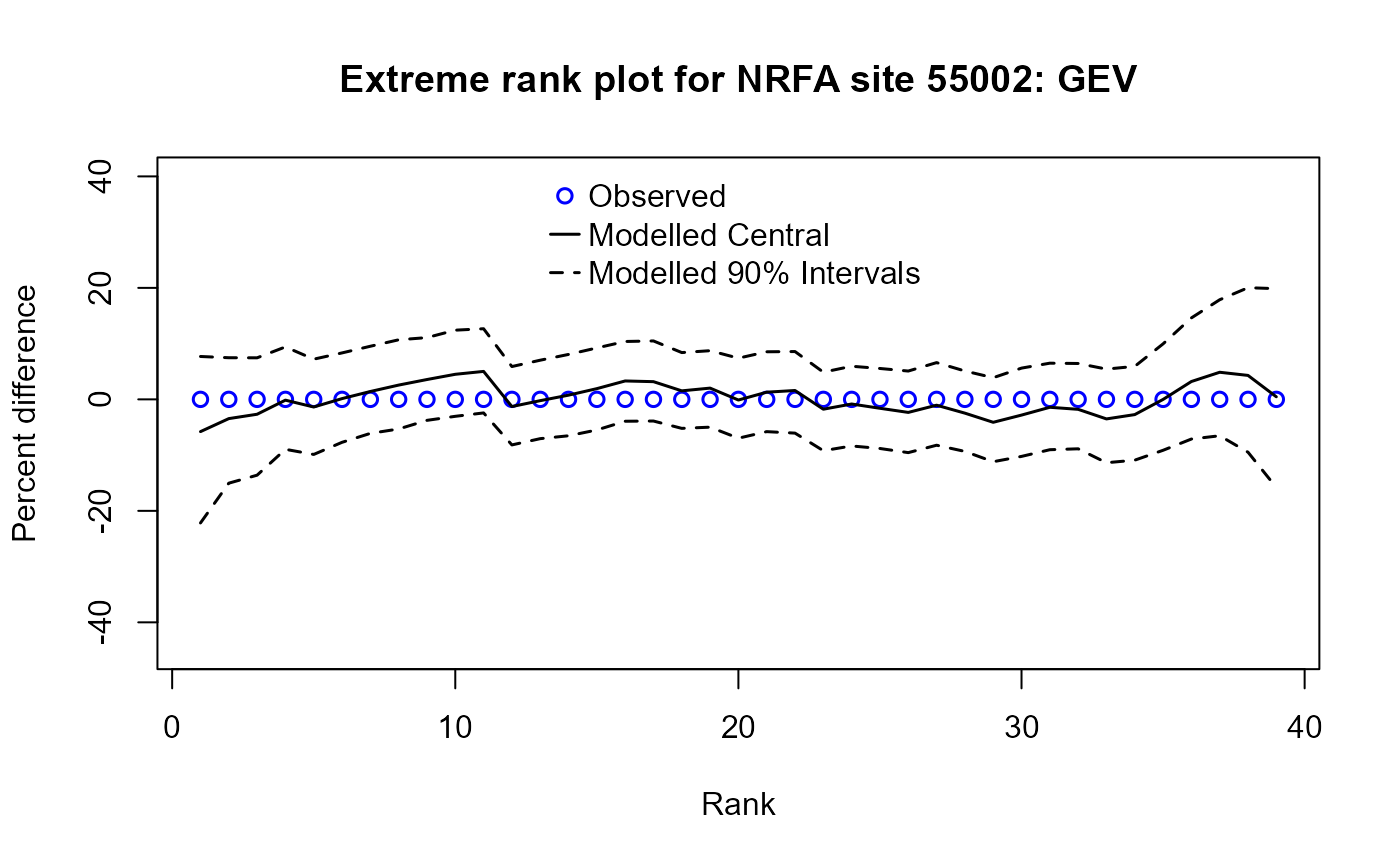
# Generate an extreme value plot for the AMAX data for NRFA site 55002 and the GEV
# distribution and set a user-defined title (using the 'Title' argument)
EVPlot(AM.55002$Flow, dist = "GEV", Title = "Extreme value plot for NRFA site 55002: GEV")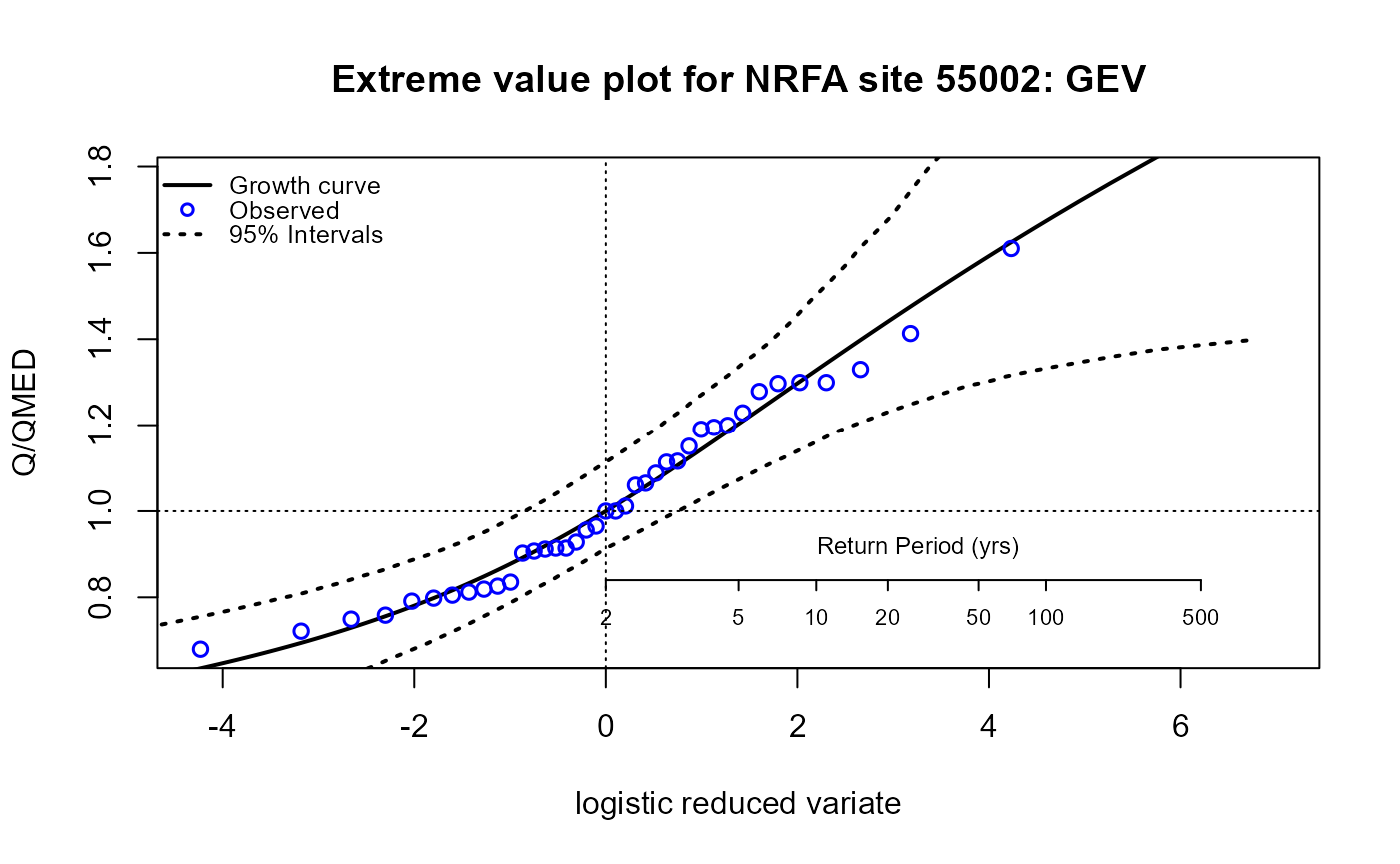
As an example, we can estimate the 100-year flow. Then, estimate the return period of the maximum observed flow. Make sure to select the “Flow” column.
# Estimate the 100-year flow directly from the AMAX data for NRFA site 55002 using
# the GEV distribution
GEVAM(AM.55002$Flow, RP = 100)
#> [1] 718.969

# Estimate the return period of the maximum observed flow directly from the AMAX
# data using the GEV distribution
GEVAM(AM.55002$Flow, q = max(AM.55002$Flow))
#> [1] 65.4758
We can also estimate the parameters of the GEV from the data, using the default L-moments, and estimate quantiles as a function of return period (and vice versa) from user input parameters.
# Estimate the parameters of the GEV distribution from the AMAX data for NRFA site 55002
GEVPars55002 <- GEVPars(AM.55002$Flow)

# View the parameters
GEVPars55002
#>        Loc    Scale      Shape
#> 1 399.6551 82.72261 0.07862905

# Estimate the 75-year flow using these GEV parameters
GEVEst(loc = GEVPars55002$Loc, scale = GEVPars55002$Scale, shape = GEVPars55002$Shape, RP = 75)
#> [1] 702.106
If we derive L-moments for the site, we can then estimate growth
factors. The LMoments() function does this. We can also
calculate L-CV and L-skew separately using the Lcv() and
LSkew() functions.
# Estimate the 75-year GEV growth factor from the L-moments for the AMAX data for
# NRFA site 55002
GEVGF(lcv = Lcv(AM.55002$Flow), lskew= LSkew(AM.55002$Flow), RP = 75)
#> [1] 1.634548
We can estimate the 75-year flow by combining this latter result with QMED (the median of the AMAX record).
# Estimate the 75-year flow by multiplying the growth factor by the median AMAX flow
GEVGF(lcv = Lcv(AM.55002$Flow), lskew= LSkew(AM.55002$Flow), RP = 75) * median(AM.55002$Flow)
#> [1] 704.4903
This gives a different 75-year flow estimate from the more direct estimate using the GEV parameters. This is because the former calculates the T-year peak directly, whereas the latter assumes a distribution scaled by the index flood.
Peaks over threshold
A peaks over threshold (POT) series can also be obtained from a time
series using the POTextract() function. A daily sample of
the Thames at Kingston flow is included in the package for example
purposes (the data frame ThamesPQ). The
POTextract() function can be used on a single vector or a
data frame, with dates in the first column and the time series of
interest in the second. In the ThamesPQ data frame, the
Thames flow is in the third column and the date in the first. Therefore,
the POT series can be extracted as follows:
# Extract a POT series from the Thames at Kingston daily mean flow data, selecting
# the first and third columns from the ThamesPQ data frame which contain the date
# and flow data respectively. The threshold is set as the 90th percentile.
POT.Thames <- POTextract(ThamesPQ[, c(1, 3)], thresh = 0.9)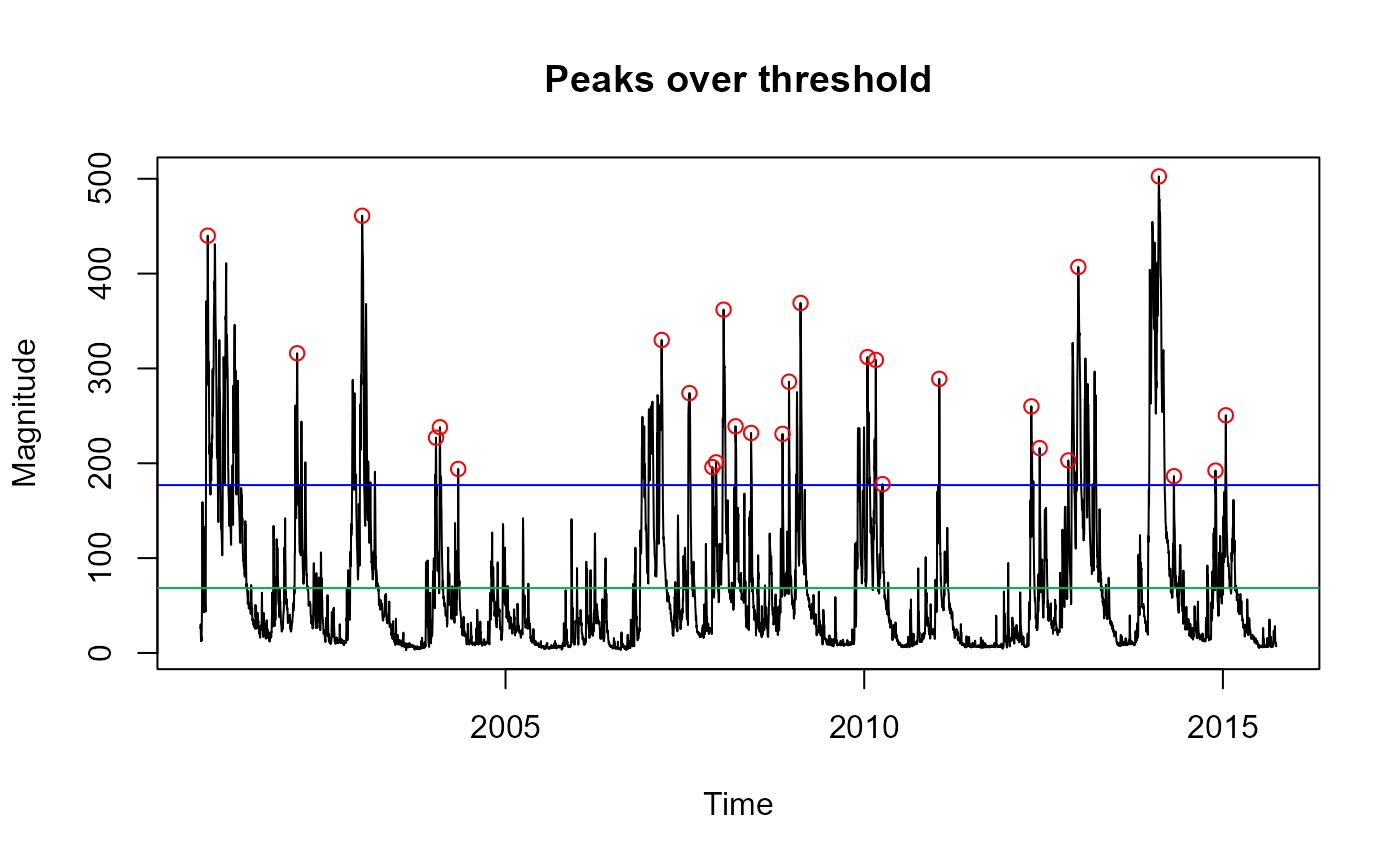
#> [1] "Peaks per year: 1.867263"

# View the output
POT.Thames
#>           Date  peak
#> 3   2000-11-07 440.0
#> 25  2002-02-05 316.0
#> 34  2003-01-02 461.0
#> 40  2004-01-13 227.0
#> 41  2004-02-02 238.0
#> 43  2004-05-05 194.0
#> 56  2007-03-07 330.0
#> 58  2007-07-26 274.0
#> 59  2007-11-20 196.0
#> 62  2007-12-09 201.0
#> 64  2008-01-16 362.0
#> 66  2008-03-17 239.0
#> 67  2008-06-04 232.0
#> 68  2008-11-11 231.0
#> 69  2008-12-14 286.0
#> 72  2009-02-11 369.0
#> 77  2010-01-18 312.0
#> 82  2010-03-01 309.0
#> 83  2010-04-04 178.0
#> 84  2011-01-18 289.0
#> 85  2012-05-01 260.0
#> 87  2012-06-12 216.0
#> 88  2012-11-05 203.0
#> 91  2012-12-26 407.0
#> 106 2014-02-09 502.5
#> 110 2014-04-27 186.4
#> 111 2014-11-24 192.3
#> 113 2015-01-16 250.6
This produces a figure showing the daily mean flow data with peaks over the threshold shown as red circles. The blue line is the threshold, and the green line is the mean flow. Independent peaks are chosen above the threshold. If peaks are separated by a drop below the mean flow (green line), they are considered independent. More details can be found in the function’s help file (including other options for defining independence and how to rename axis labels and the plot title).
Note that you can also use the POTt() function for
extracting peaks over threshold. It works significantly faster, but only
has the option of separating peaks by the number of timesteps.
The POT approach is similar to the AMAX approach, except that we need
to convert from the POT RP scale to the annual RP scale. To do so, the
functions have a peaks per year (ppy) argument. The
POTextract() function provides the number of peaks per year
(in this case, 1.867). To estimate the associated 100-year daily mean
flow peak, the GenPareto function can be used as follows:
# Estimate the 100-year flow for the Thames at Kingston using the extracted POT series
GenParetoPOT(POT.Thames$peak, ppy = 1.867, RP = 100)
#> [1] 605.432
Uncertainty
Methods for quantifying aleatoric (sampling) uncertainty are provided here for three estimation methods: single-site, gauged pooling, and ungauged pooling. The uncertainty is predicated on forming a sampling distribution for the statistic of interest, and in the three cases (single site, gauged pooling, and ungauged pooling), it is done using bootstrapping. In the pooling approaches (gauged and ungauged), the whole pooling group is bootstrapped, and the weighted estimates provided on every iteration.
Single-site
Extract an annual maximum sample with the following code.
# Extract the AMAX for NRFA site 55002
AM.55002 <- GetAM(55002)
The uncertainty for the 100-year flow can be estimated using the
Bootstrap() function. The 95% confidence intervals are
provided by default, but this can be adjusted using the
Conf argument. The lower limit is provided in the ‘Lower’
column and the upper limit in the ‘Upper’ column.
Note that the Bootstrap() function can also be applied
for any function/statistic, and the sampling distribution developed can
be returned.
# Estimate uncertainty for the GEV-estimated 100-year flow
Bootstrap(AM.55002$Flow, Stat = GEVAM, RP = 100)
#>   Mean Lower Upper
#> 1  709   609   827
Ungauged pooling
The Uncertainty() function can be used for the pooled
estimates to quantify the sampling uncertainty. The estimated QMED and
the pooling group are required. Furthermore, the factorial standard
error needs to be provided for the ungauged case, using the
fseQMED argument (the default is 1.5). Note that by default
the generalised logistic distribution is selected for the estimates, but
this can be changed.
The following example to estimate uncertainty for the ungauged pooled
estimates for NRFA site 55002 uses the catchment descriptors object
created earlier (CDs.55002). This provides a dataframe with
return period in the first column and Factorial Standard Error (FSE) in
the second. For confidence intervals you can divide and multiply your
estimates for each return period by the FSE. For 95% intervals do the
same but raise the FSE to the power of 1.96.
# Estimate QMED for site 55002 from catchment descriptors using two donors
QMEDEst <- QMED(CDs.55002, DonorIDs = c(55007, 55016))

# Create an ungauged pooling group for site 55002
PoolUG.55002 <- Pool(CDs.55002, exclude = 55002)

# Estimate the uncertainty of the pooling results
Uncertainty(PoolUG.55002, QMEDEstimate = QMEDEst)
#>      RP    FSE
#> 1     2 1.5000
#> 2     5 1.5104
#> 3    10 1.5213
#> 4    20 1.5363
#> 5    30 1.5473
#> 6    50 1.5640
#> 7    75 1.5797
#> 8   100 1.5922
#> 9   200 1.6274
#> 10  500 1.6854
#> 11 1000 1.7383
Gauged pooling
The gauged case is similar to the above, but the Gauged
argument is set to TRUE, and there is no need to set
QMEDEstimate; it is derived from the observed AMAX if
Gauged = TRUE.
It is important to note that when Gauged equals
TRUE, the top site in the pooling group is assumed to be
the “gauged” site of interest. This will happen by default because the
similarity distance measure should be zero - assuming the that “gauged”
site is within the NRFAData data frame.
The following example uses the gauged pooling group we previously derived:
# Create a gauged pooling group for site 55002
Pool.55002 <- Pool(CDs = CDs.55002, exclude = c(8010, 76017))

# Estimate the uncertainty of the pooling results
Uncertainty(Pool.55002, Gauged = TRUE)
#>      RP    FSE
#> 1     2 1.0576
#> 2     5 1.0567
#> 3    10 1.0575
#> 4    20 1.0598
#> 5    30 1.0619
#> 6    50 1.0653
#> 7    75 1.0688
#> 8   100 1.0716
#> 9   200 1.0796
#> 10  500 1.0927
#> 11 1000 1.1042