The ReFH() function
This quick guide provides an overview of how to generate a design hydrograph using the ReFH method. It is assumed that the reader has knowledge of the theory of the ReFH method; this guide is intended to demonstrate how to use the UKFE package rather than to explain the method.
The ReFH() function is designed for flexibility and each
parameter of the model, along with the inputs and initial conditions,
can be user-defined. By default, when catchment descriptors are
provided, the ReFH function uses these descriptors to estimate the
parameters of the ReFH model, and an estimate of the two-year rainfall
for the critical duration (the two year rainfall is approximated from
the RMED catchment descriptors). When catchment descriptors are applied,
individual parameters and settings can still be adjusted by the user and
these adjustments override the estimates from the catchment descriptors.
Further details can be found in the function’s help file.
This function applies the ReFH model as specified by Kjeldsen (2007). The ReFH model has since been updated to address some of the limitations. The updated version(s), known as ReFH2, was developed by Wallingford Hydro Solutions (2019) and is available for a licence fee. Henceforth, the original model is denoted ReFH1, and the term ‘ReFH’ is used when the comment applies to the original and updated versions.
The ReFH outputs are commonly used only to derive a reasonable hydrograph shape. This shape is then scaled to match the peak flow estimate derived using other methods (usually FEH statistical methods). An example of doing this with the function is provided below. There is no automated way of doing so within the function but ReFH parameters can be calibrated using observed rainfall and data to replicate storm events.
Assumptions and limitations of the ReFH1 model are provided at the bottom after the example of how to derive a design hydrograph.
Derive a design hydrograph using the ReFH method
In the following example, the ReFH() function is used to derive a design hydrograph, i.e., a hydrograph shape scaled to our design flood estimate (assuming the site to be ungauged). The default use of ReFH() with the catchment descriptors provides the rainfall-runoff outputs for an estimate of the two-year design rainfall event:
# Obtain catchment descriptors for NRFA gauge 55002
CDs.55002 <- GetCDs(55002)

# Obtain outputs of the ReFH model from catchment descriptors for a default 2-year
# rainfall event
ReFHResult55002 <- ReFH(CDs.55002)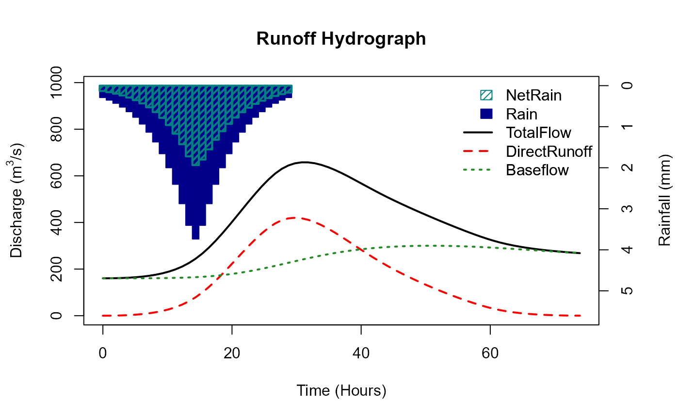
# print to console
ReFHResult55002
#> [[1]]
#>   AREA   TP Duration   BR   BL Cmax Cini BFini Season Depth Timestep
#> 1 1890 12.8     29.8 1.13 62.6  306  138   160 winter  41.3 1.025998
#>   DurationFinal PeakFlow
#> 1          29.8      658
#>
#> [[2]]
#>     Time_hrs  Rain NetRain  Runoff Baseflow TotalFlow
#> 1   0.000000 0.290   0.131   0.000      160       160
#> 2   1.025998 0.353   0.160   0.141      160       161
#> 3   2.051997 0.430   0.195   0.593      160       161
#> 4   3.077995 0.523   0.238   1.420      160       162
#> 5   4.103993 0.635   0.290   2.710      161       163
#> 6   5.129992 0.771   0.354   4.570      161       165
#> 7   6.155990 0.936   0.432   7.110      161       168
#> 8   7.181988 1.130   0.527  10.500      161       171
#> 9   8.207987 1.370   0.644  14.900      161       176
#> 10  9.233985 1.660   0.786  20.600      161       182
#> 11 10.259984 2.000   0.960  27.700      162       190
#> 12 11.285982 2.400   1.170  36.800      162       199
#> 13 12.311980 2.880   1.430  48.100      163       211
#> 14 13.337979 3.400   1.720  62.200      164       226
#> 15 14.363977 3.740   1.940  79.200      165       245
#> 16 15.389975 3.400   1.800  99.500      167       266
#> 17 16.415974 2.880   1.550 123.000      169       292
#> 18 17.441972 2.400   1.320 150.000      171       321
#> 19 18.467970 2.000   1.110 178.000      174       352
#> 20 19.493969 1.660   0.931 208.000      177       385
#> 21 20.519967 1.370   0.777 239.000      181       420
#> 22 21.545965 1.130   0.647 269.000      186       455
#> 23 22.571964 0.936   0.537 299.000      190       489
#> 24 23.597962 0.771   0.445 328.000      196       523
#> 25 24.623960 0.635   0.368 354.000      201       555
#> 26 25.649959 0.523   0.304 377.000      207       584
#> 27 26.675957 0.430   0.250 396.000      214       610
#> 28 27.701956 0.353   0.206 410.000      220       630
#> 29 28.727954 0.290   0.170 418.000      227       645
#> 30 29.753952 0.000   0.000 420.000      234       654
#> 31 30.779951 0.000   0.000 418.000      240       658
#> 32 31.805949 0.000   0.000 411.000      247       658
#> 33 32.831947 0.000   0.000 401.000      253       654
#> 34 33.857946 0.000   0.000 388.000      258       647
#> 35 34.883944 0.000   0.000 373.000      264       637
#> 36 35.909942 0.000   0.000 357.000      269       626
#> 37 36.935941 0.000   0.000 339.000      273       612
#> 38 37.961939 0.000   0.000 320.000      278       598
#> 39 38.987937 0.000   0.000 301.000      282       583
#> 40 40.013936 0.000   0.000 283.000      285       567
#> 41 41.039934 0.000   0.000 264.000      288       552
#> 42 42.065932 0.000   0.000 246.000      291       537
#> 43 43.091931 0.000   0.000 229.000      293       522
#> 44 44.117929 0.000   0.000 213.000      295       508
#> 45 45.143928 0.000   0.000 197.000      296       494
#> 46 46.169926 0.000   0.000 183.000      298       480
#> 47 47.195924 0.000   0.000 169.000      299       467
#> 48 48.221923 0.000   0.000 155.000      299       455
#> 49 49.247921 0.000   0.000 142.000      300       442
#> 50 50.273919 0.000   0.000 130.000      300       430
#> 51 51.299918 0.000   0.000 117.000      300       418
#> 52 52.325916 0.000   0.000 106.000      300       406
#> 53 53.351914 0.000   0.000  94.500      299       394
#> 54 54.377913 0.000   0.000  83.600      299       382
#> 55 55.403911 0.000   0.000  73.200      298       371
#> 56 56.429909 0.000   0.000  63.300      297       360
#> 57 57.455908 0.000   0.000  53.800      296       350
#> 58 58.481906 0.000   0.000  45.000      295       340
#> 59 59.507904 0.000   0.000  36.900      293       330
#> 60 60.533903 0.000   0.000  29.700      292       321
#> 61 61.559901 0.000   0.000  23.700      290       314
#> 62 62.585900 0.000   0.000  18.600      288       307
#> 63 63.611898 0.000   0.000  14.500      287       301
#> 64 64.637896 0.000   0.000  11.100      285       296
#> 65 65.663895 0.000   0.000   8.400      283       291
#> 66 66.689893 0.000   0.000   6.220      281       287
#> 67 67.715891 0.000   0.000   4.490      279       284
#> 68 68.741890 0.000   0.000   3.140      277       280
#> 69 69.767888 0.000   0.000   2.100      275       278
#> 70 70.793886 0.000   0.000   1.320      274       275
#> 71 71.819885 0.000   0.000   0.752      272       273
#> 72 72.845883 0.000   0.000   0.364      270       270
#> 73 73.871881 0.000   0.000   0.122      268       268
The output that is printed to the console is a list with two elements. The first element is a data frame of parameters, settings, initial conditions, the catchment area, and peakflow. The second is a data frame with the following columns: Time, Rain, NetRain, Runoff, Baseflow and TotalFlow. A runoff hydrograph plot is also produced.
Scaled ReFH hydrograph
To scale the hydrograph to the design flow estimate, the results from the ungauged pooling can be used (assuming this is for the ungauged case). We can use the estimate from the FEH statistical analysis vignette:
# Create an ungauged pooling group for site 55002
PoolUG.55002 <- Pool(CDs.55002, exclude = 55002)

# Estimate QMED for site 55002 using catchment descriptors and two donor gauges
CDsQmed.55002 <- QMED(CDs.55002, DonorIDs = c(55007, 55016))

# Estimate design flows using the above pooling group and QMED
Results55002 <- PoolEst(PoolUG.55002, QMED = CDsQmed.55002, CDs = CDs.55002)
The results are in the form of a list. The first element provides the return levels, and the 100-year flow estimate is in the 8th row in the second column. We’ll make it an object and use it to scale the hydrograph:
# Extract the 100-year flow estimate (the [[1]] denotes the first element of the list - which is a dataframe, then [8,2] is the 8th row and 2nd column of that dataframe)
Q100.55002 <- Results55002[[1]][8, 2]

# Obtain the final flow outputs of the ReFH model from catchment descriptors for a default 2-year
# rainfall
TotalFlow <- ReFHResult55002[[2]]$TotalFlow

#Scale this by dividing by the maximum of the flow
ScaledFlow <- TotalFlow / max(TotalFlow)

#Multiply the scaled flow by our peak flow estimate and plot
plot(ScaledFlow * Q100.55002, type = "l", lwd = 2, ylab = "Discharge (m3/s)", xlab = "Time (hours)")
Exporting results
For use outside of ‘R’, these outputs can be saved as objects and then written to CSV files:
# Save the ReFH design hydrograph to an object called 'DesignHydro55002'.
DesignHydro55002 <- ScaledFlow * Q100.55002

# Write to csv
write.csv(DesignHydro55002, "my/file/path/DesHydro55002.csv", row.names = FALSE)
Note in these examples that row.names = FALSE in the
write.csv() function: our data has no row names, so this
prevents an index column being added to the CSV.
ReFH function as a flexible design rainfall funoff tool
By default this ReFH function is the orginal ReFH model as described by Kjeldsen (2007). Also by default the Flood Studies Report (FSR) rainfall profiles are applied. However, it has many options, including the ability to provide rainfall or choose a randomised profile. Furthermore, the main components can be adjusted such as the unit hydrograph shape, the baseflow, and the loss. For example, if you set UHShape = “FSR”, BR = 0, and Loss = 0.5 (or some other proportion), the FSR/FEH design rainfall runoff model is the result. You can also set UrbanLoss = TRUE, and the urban loss model as used in the ReFH2.3 software is applied.
ReFH.FSR <- ReFH(CDs.55002, RainProfile = "Centre", UHShape = "FSR", Loss = 0.3, BR = 0)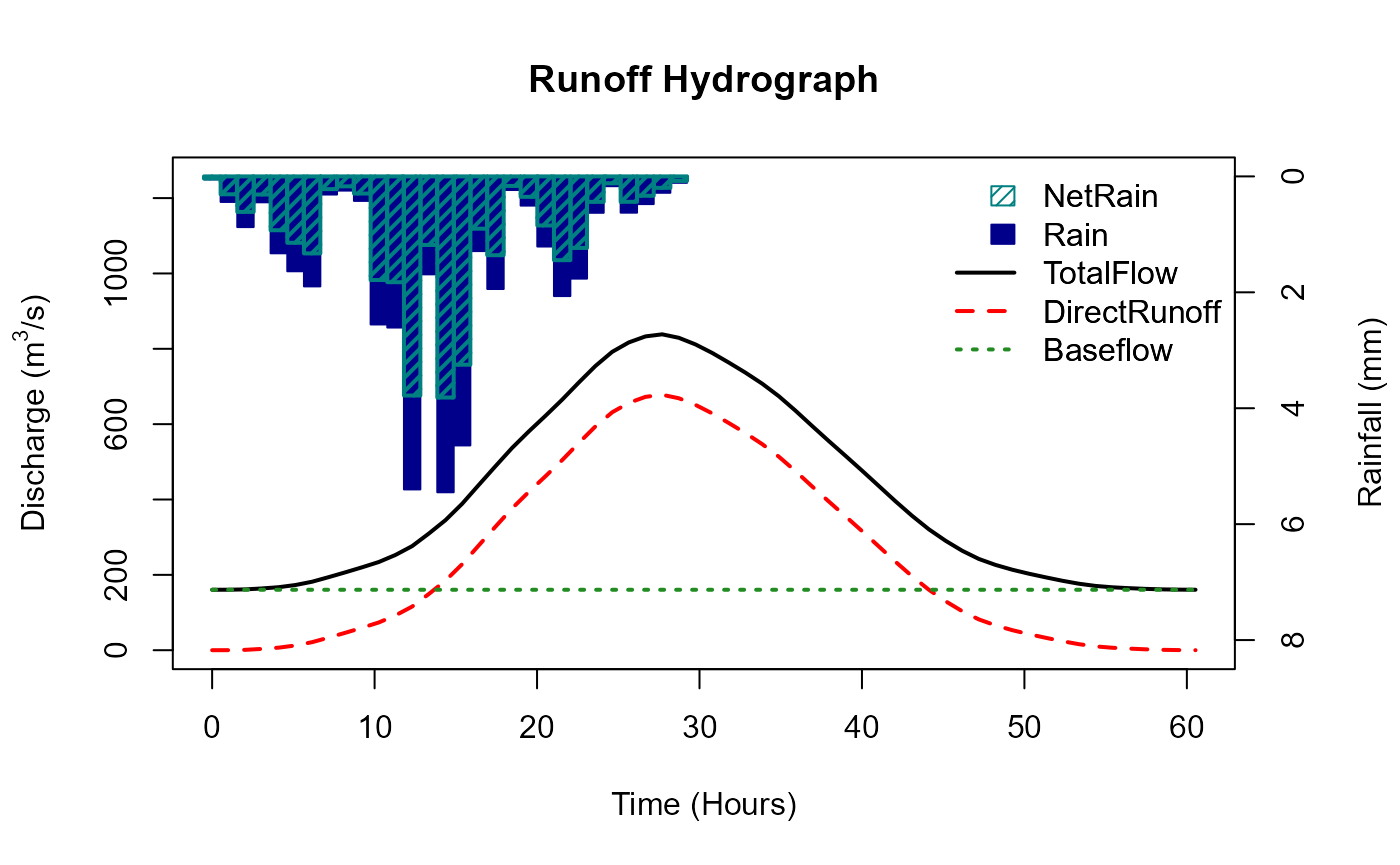
ReFH overview, assumptions and limitations
The ReFH model has three components that conceptualise the catchment process.
Model structure:
- A loss model to account for hydrological processes such as evaporation, soil moisture storage, groundwater recharge and interception losses.
- A unit hydrograph-based routing model to distribute the net rainwater over time at the catchment outlet (runoff).
- A baseflow model which determines the proportion of the runoff which becomes baseflow recharge and specifies the exponential decay of the river flow once the net rainfall has been routed through the catchment outlet.
Loss model
The loss model quantifies, for each timestep of rainfall, the proportion of the rain that is effective (the rain that forms the runoff hydrograph). It does so by assuming a maximum catchment soil moisture capacity in mm (Cmax) and an initial catchment soil moisture content in mm (Cini). The original ReFH report (Kjeldsen, 2007) suggests that the Cini / Cmax (Cini divided by Cmax) can be conceptualised as the initial proportion of the catchment that is saturated, and the initial rainfall on this saturated area will form the storm hydrograph. It is assumed that the proportion of rain becoming effective is the same as this saturated proportion.
As rainfall is added, catchment soil moisture increases and Cini / Cmax becomes Ct / Cmax, i.e. the soil moisture for the given timestep divided by the Cmax is the proportion of rain for each timestep which becomes effective.
Runoff routing model (unit hydrograph)
The unit hydrograph (UH) model is a well-established method for routing effective rainfall to the catchment outlet (Sherman, 1932). There are a number of assumptions:
- There is a direct proportional relationship between the effective rainfall and the surface runoff.
- The property of superposition. That is, if two successive amounts of
effective rainfall, then the surface runoff is the sum of the two
associated unit hydrographs (the second one being ahead by one
timestep).
- The UH does not change over time.
- The UH shape is the same for all catchments. Only the time to peak and the associated base of the UH changes between catchments.
- The catchment rainfall is spatially homogeneous.
- The rainfall in a given timestep has a constant intensity.
Baseflow model
The baseflow model assumes that the saturated area of the catchment that produces surface runoff is the same area that also produces the baseflow recharge. The assumption is that the ratio of recharge to runoff is fixed (the BR parameter). A further parameter, baseflow lag (BL), ensures that the resulting baseflow hydrograph is lagged behind that of the runoff hydrograph (effectively providing a slow flow component). However, this baseflow model does not consider the volume of rainfall directly in the same way the unit hydrograph component does. The resulting baseflow hydrograph is in addition to the runoff hydrograph volume and is calculated as a proportion of it. This means that the volume of the total hydrograph minus initial baseflow is greater than the net/effective rainfall. For the most part, this is not a significant problem because it is assumed that some of the remaining volume of the rainfall makes up the difference. However, if the proportion of effective rainfall is closer to one, the volume of the hydrograph can be greater than the gross/total input of rainfall. This will almost certainly not happen unless the event duration is considerably longer than recommended and only in catchments with a high initial proportion of saturation (due to low BFIHOST and high PROPWET). However, this ReFH function has a WaterBalance argument and setting it to TRUE means that the water balance cannot be invalidated because BR is capped such that BR = (1/NetProp)-1, NetProp is the proportion of effective rainfall.
Use cases for the ReFH() function
There are three primary use cases:
- A flexible tool to model the catchment response to event rainfall.
- A tool for estimating the T-year flow as a function of the T-year rainfall.
- To develop a plausible hydrograph shape for scaling to peak flow estimates (usually for the purposes of developing a model boundary).